Plotting Health Data

I’m well aware that this article is in danger to get into an apples vs. oranges comparison. Bookshelves can be filled with books about Wolfram’s Mathematica and JupyterLab/Jupyter, many of them demonstrating how very different the software tools are. Mathematica is a commercial software package, JupyterLab is an open-source web application that is a front end to a variety of interactive compute kernels. And yet, the problems they help to solve do overlap. So it seems fair to compare those products for an application that both are well suited to handle and ignore the vast differences the software packages have in other areas.
The Notebook Interface for Technical Computing

The main draw to Mathematica arguably always has been the notebook interface. In 1988 Mathematica pioneered the use of an interactive computational notebook to explore problems through technical computing. I’m very much a believer in that concept, and once in a while, I like to see how much progress open source software has made to provide comparable functionality.
I experimented with the Jupyter notebook in the past. However, I found its user interface to be inferior to Mathematica; nothing else stood out to justify investing more time. Then two things happened. JupyterLab, advertised as the next generation user interface, entered beta release status[1] and Julia, a programming language I had kept an eye on for a while achieved the 1.0 release status a little later, promising a stable interface from here on forward[2]. Since Julia can be used as the kernel for which JupyterLab serves as the front end, it was time to take a closer look[3].
Getting Software Installed
Mathematica is an easy install; download the installer and double-click. For JupyterLab, installing Anaconda is the easiest way to get started. The Anaconda installer also installs IPython, a Python kernel for JupyterLab. To get access to Julia requires a separate step. The Julia language itself has to be installed, followed by the installation of IJulia to make JupyterLab aware of Julia. IJulia is a package, and the first notable difference between Mathematica and JupyterLab jumps out here, as Mathematica provides a single integrated software package that comes with all the bells and whistles. No hunting on the Internet for packages that add the functionality useful for a given purpose. Spoiler alert: This will be a recurring theme.
Get some Data to Plot
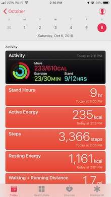
I’m getting my data from Apple’s Health App. My phone and my Watch are constantly dumping data into it, so there is lots to visualize. QS Access is a tool I found that extracts the data from the Health App and saves it in a CSV formatted file. Mathematica can read such a file with built-in functionality. Both Python and Julia need additional packages. Specifically, for Julia I made use of CSV, DataFrames, Query, Dates and Gadfly. Note the challenge here, figuring out which packages to select. There are competing packages that provide similar functionality with varying degree of support. Some packages have direct support for each other, which is how I ended up with that list. Starting from DataFrames, its documentation pointed me at the CSV and the Query package. Gadfly is a plotting package promising a tight integration with the DataFrame package as well. Overall, it requires quite a bit of effort to figure out what packages to use compared to a tool like Mathematica. Working with Python is also less cumbersome than Julia as it provides a large standard library that includes much of the functionality; issues with package compatibility do not arise.
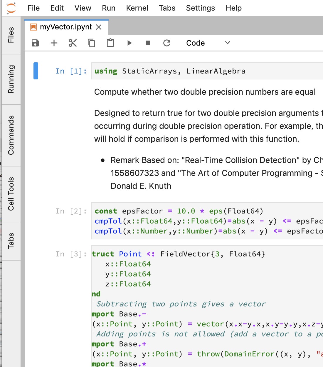
JupyterLab and Julia
Importing CSV formatted data is straightforward. Simply load the CSV package and add one line of code to read the CSV file. We can display a table with the variables it found plus some summarizing information:
The CSV file contained a lot of data, from calories used to steps climbed. For this blog post, I wanted to display only blood pressure, which can be extracted using functionality provided by the Query package. It makes it easy to target the columns containing the data of interest. This is also an excellent opportunity to convert the date, which was imported as a string, into a datetime construct that gives Julia more context to help with plotting the timeline.

Thanks to the tight integration of the DataFrames package with the plotting tool Gadfly, plotting the extracted data is a couple of lines of code:

JupyterLab and Python
Let’s walk through the process again, this time using Python 3 as the kernel for JupyterLab. I didn’t look for a package similar to DataFrames that would provide a higher level interface to the data, but instead opted to work directly with Python data structures:

Next, we need to delete the header, turn the dates into datetime structures and the strings containing the values into floating point values before we hand the data to the plot function.

Note that I had to write a little more code compared to what I was able to do with Julia, most likely because opted for dealing with low-level Python data structures directly instead of investigating third party Python packages that could have made it a little easier.
Mathematica
Importing CSV datasets into Mathematica takes just a few steps.

Again we want to drop all but the blood pressure values. With that accomplished, the data is converted into a TimeSeries. A TimeSeries is a high level construct in Mathematica that provides a lot of functionality on time-dependent data. Not only can we pass it to a function to create a diagram, but the TimeSeries understands how to handle irregularly sampled data, missing values, and it serves as input to many tools for processing time series, e.g., moving averages to name one that I use.
Here is the Mathematica code that accomplishes all that and creates a plot similar to the examples written in Julia and Python:

Conclusion
As I mentioned in the introduction, this was an exercise for me to see how useful the JupyterLab notebook is in comparison to Mathematica, based on a particular example. It is somewhat difficult to evaluate only the notebook interfaces as using them means interacting with a programming language underneath, which can influence the experience a lot. Just compare the Julia and Python code above, both executed from the JupyterLab notebook. Still, I have some conclusions. The notebook interface in JupyterLab is arguably very well done, and after finding the right packages to extend Julia with, the functionality I needed to go from data in a CSV file to a plot can be written at a high level that makes it fun to use. For the example here, the Jupyter notebook with Julia as the kernel can hold its own against Mathematica.
A big minus is that Julia’s standard library is small compared to what Python or Mathematica provide out of the box. That means a healthy ecosystem of open source packages that are well designed and supported is a necessity. At the current time that is the downside of Julia. I ran into several packages that weren’t updated to the latest Julia release and thus incompatible with my installation. In fairness, the 1.0 release that promises language stability was just released; the situation might improve going forward. Still, compare that to Mathematica, for which you will be hard pressed to find programs written a decade ago that won’t run with the current release.
Picture Credits:
- apple vs. organges courtesy of MicroAssist, provided under the Attribution-ShareAlike 2.0 Generic (CC BY-SA 2.0) license
- Mathematica displayed on Macintosh courtesy of OrdinaryArtery - Own work, CC BY-SA 4.0